Bioinformatics steps in RNA sequencing data analysis (Tutorial)

Quantifying gene expression and identifying transcripts that are differentially expressed between two sets of samples is an important approach in modern biotechnology. RNA-seq analysis based on next-generation sequencing (NGS) data is the gold standard for the analysis of gene expression at the level of the whole transcriptome. RNA-seq involves isolation of total RNA from tissues or cells of interest followed by the construction of DNA libraries and sequencing of these libraries using a next-generation sequencing instrument (Fig 1).

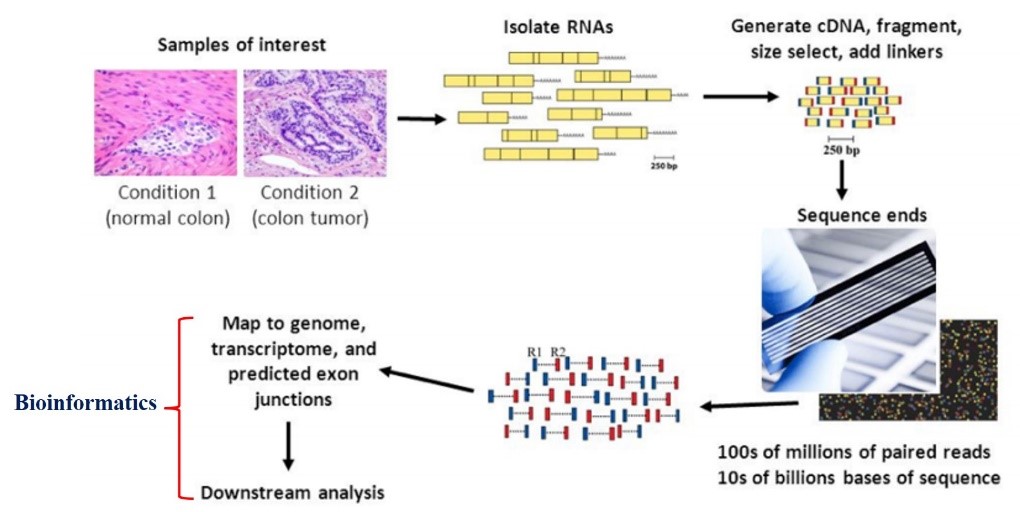Fig1 Fig 1. RNA sequencing steps (From Griffith et al. (2015))

In this tutorial, we explain the different bioinformatics steps involved in the analysis of RNA seq data to find the differentially expressed genes in two distinct sets of samples. Fig 2 shows the current workflow of bioinformatics analysis of RNA seq data.

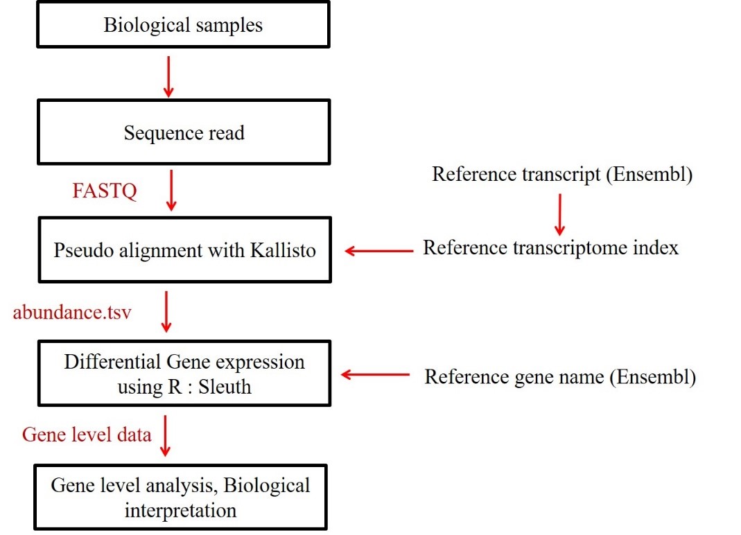Fig2 Fig 2. Current RNA seq analysis work flow

Data selection for the analysis

Drosophila is a fruit fly belonging to the family Drosophilidae. Drosophila melanogaster, one species of drosophila, has been widely used as a model organism in developmental biology. A study has been conducted by Allada Lab to understand the molecular mechanisms by which discrete circadian clock neurons program a homeostatic sleep center Full Text. In normal cycles of day and night, Drosophila exhibits morning and evening peaks of activity, which are controlled by two different groups of neurons in the brain. In this study, RNA sequence has been done and collected the data from morning and evening cells. There are 12 samples in this study and all are deposited in the Gene Expression Omnibus (GEO) with an accession number GSE186076 GEO accession. In this tutorial, we are looking at only 6 samples Morning control (3 samples MC1, MC2, MC3) and Evening control (3 samples EC1, EC2, EC3). We select these data set because these are some special cases that will be explained in the proceeding sections. We aim to perform RNA seq analysis on these data and find out differentially expressed genes in Morning and evening cells.

I. Download the RNA seq raw data (fastq, fasta…) from the public data base.

There are many methods are exist to download raw data from the public database. Here I am describing one of the easiest methods to download the data. Users can use any method to download the data.

Note: Raw data are usually big (normally GBs). If the user is not interested in downloading the data or your internet connection has only limited bandwidth, you can skip this downloading step. Anyway, I am providing the Kallisto output here and users can download it directly from the repository and perform sleuth analysis (Differential gene expression analysis).

Downloading steps 1) Go to the European Nucleotide Archive (ENA) website 2) In the search tab on the top right, enter the GEO accession number GSE186076

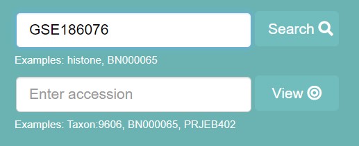Fig3 Fig 3

3) ENA provide following search results

Fig4 Fig 4

4) Click on the SRP341965 tab, you will be directed to following page

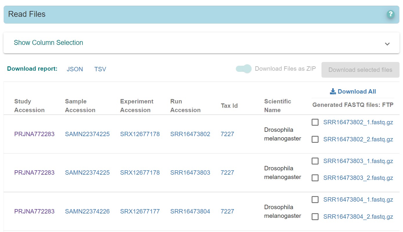Fig5 Fig 5

Now user can download all the files using Download All option or selected files by checking the box near the files.

Note: In this example there are two files per each entry, for example SRR**_1.fastq.gz & SRR**_2.fastq.gz. These are paired end sequencing (pair-1, pair-2). Kaliisto analysis is different for paired end sequencing and single end sequencing. I will explain it well in the kallisto analysis section.

In this tutorial we are only interested on EC and MC samples. When you looking at the read file window above, samples names are missing, which is difficult to understand the users. So if you need the sample names click on the ‘show column section’ tab and check the ‘sample_title’ box. Then slide the window, you can see the samples name on the right. 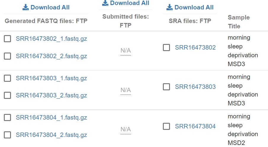Fig6 Fig 6

Now you can easily identify the samples.

5) Select only the EC and MC sample (Evening control non-sleep deprived EC1/EC2/EC3, Morning control non-sleep deprived MC1/MC2/MC3).

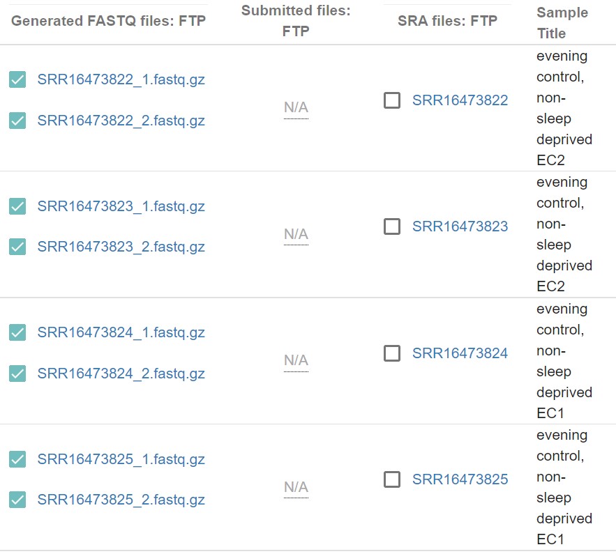Fig7 Fig 7

Note: User can see that, two entries have the same sample title (eg: evening control, non-sleep deprived EC2, evening control, non-sleep deprived EC2). These two entries are the sequencing data of the same samples but, data is split into these two entries. For example, SRR16473822_1.fastq.gz and SRR16473823_1.fastq.gz are the pair-1 end sequencing fastq files of the sample EC2 and SRR16473822_2.fastq.gz and SRR16473823_2.fastq.gz are the pair-2 end sequencing fastq files of the same sample EC2. Kaliisto analysis does not required to combine them together. I will explained it in details in the kallisto analysis section how to process these kind of data. This is what I stated at the beginning that these data sets are special case!!!!

6) Click on the ‘Download selected files’ tab to start download the fastq files. Files are downloaded in the zip file format. Unzip it and extract the files.

Now you have fastq files (raw RNA seq reads) with you. Next steps is to align the raw reads to a reference transcripts using the software Kallisto.

II. Kallisto for read alignment

First steps in the RNA seq data analysis is to aligns the reads to a reference genome (Transcriptome) to find out where it belongs. 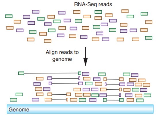Fig8 Fig 8

The softwares for sequence alignment are STAR, sailfish, Kallisto. In this tutorial we use Kallisto for the read alignment.

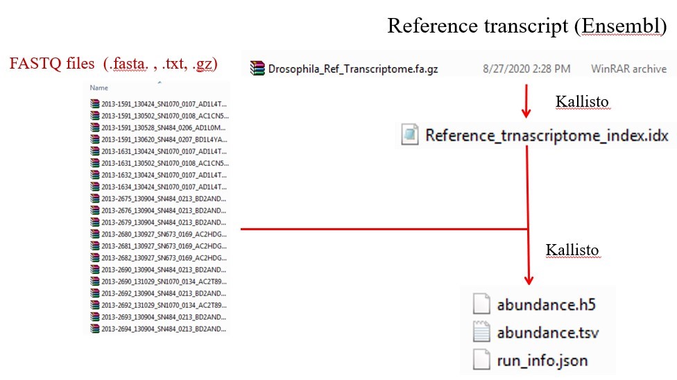Fig9 Fig 9. Work flow of read alignment using kallisto

You can download and install the kallisto software from Pacheter Lab. Installation procedure on windows OS is explained here. After the installation you can go for the kallisto analysis. Open the command window. In windows OS, search for cmd. Then type kallisto. If the installation is proper, then following lines will appear in the command window:

C:\Users\shiju>kallisto
kallisto 0.46.1

Usage: kallisto <CMD> [arguments] ..

Where <CMD> can be one of:

    index         Builds a kallisto index
    quant         Runs the quantification algorithm
    bus           Generate BUS files for single-cell data
    pseudo        Runs the pseudoalignment step
    merge         Merges several batch runs
    h5dump        Converts HDF5-formatted results to plaintext
    inspect       Inspects and gives information about an index
    version       Prints version information
    cite          Prints citation information

Running kallisto <CMD> without arguments prints usage information for <CMD>

kallisto transcriptome indices You have two option to create a transcriptome indices. Either directly download it, or generated it using reference genome using following command
```
     kallisto index -i transcripts.idx Ref_Transcriptome.fa
```
First method is the easiest method. User can download the transcriptome indices of different species from here. Download the drosophila_melanogaster.tar.gz and extract the files. There are different files on the folder, copy the file transcriptome.idx, and place on the folder containing fastq files. Now all the fastq files and transcriptome.idx files are in the same folder.

These are the samples and their corresponding fastq files

MC1

SRR16473812_1.fastq.gz, SRR16473812_2.fastq.gz, SRR16473813_1.fastq.gz, SRR16473813_2.fastq.gz

MC2

SRR16473810_1.fastq.gz, SRR16473810_2.fastq.gz, SRR16473811_1.fastq.gz, SRR16473811_2.fastq.gz

MC3

SRR16473808_1.fastq.gz, SRR16473808_2.fastq.gz, SRR16473809_1.fastq.gz, SRR16473809_2.fastq.gz

EC1

SRR16473824_1.fastq.gz, SRR16473824_2.fastq.gz, SRR16473825_1.fastq.gz, SRR16473825_2.fastq.gz

EC2

SRR16473822_1.fastq.gz, SRR16473822_2.fastq.gz, SRR16473823_1.fastq.gz, SRR16473823_2.fastq.gz

EC3

SRR16473820_1.fastq.gz, SRR16473820_2.fastq.gz, SRR16473821_1.fastq.gz, SRR16473821_2.fastq.gz

Now we can look at the sample MC1 and do the alignment using kallisto. Folder may be look like this:

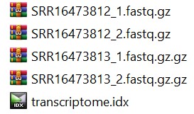Fig11 Fig 10

For pseudo alignment enter the following command in the command prompt.

Change the directory first. Locate to the folder where the fastq files and index file are stored. For example, I stored above the files in D drive with a folder name Drosophila_fastq_MC1

Type on the command line:

Cd D:\Drosophila_fastq_MC1

kallisto quant runs the quantification algorithm. The syntax for the quant command for single end sequencing reads is as below:
```
kallisto quant -i index_file -o output_folder --single -l 200 -s 20 file1.fastq.gz file2.fastq.gz file3.fastq.gz...
```

Index_file is the transcriptome indices file that is we already downloaded. In this case it is transcriptome.idx. output_folder is the folder name where we have to store the kallisto output for this sample. Good practice is giving the sample name itself. In this example appropriate output folder name is MC1. -l is the estimated average fragment length, -s is the estimated standard deviation of fragment length. Typical Illumina libraries produce fragment lengths ranging from 180–200 bp. The last parts are fastq file name which we need to quantify. However, in our case it is paired end sequence. Syntax for the quant command for paired end sequencing reads are as below:

kallisto quant -i index_file -o output_folder -b 10 pairA_1.fastq pairA_2.fastq pairB_1.fastq pairB_2.fastq

Here -b is the number of bootstrap samples required. We can now replace dummy parts with our example input. It will be look like as follows:

kallisto quant -i transcriptome.idx -o MC1 -b 10 SRR16473812_1.fastq.gz SRR16473812_2.fastq.gz SRR16473813_1.fastq.gz SRR16473813_2.fastq.gz

Note: There is space between fastq files, but not comma.

Depending on your system speed and performance, it will take some time to complete the quantification. After the successful run, kallisto output for this sample will be stored in the folder MC1. The folder will be look like as follows:

Fig12 Fig 11

Like this, finish the kallisto quant analysis for all other samples. If you want to run all the sample in one step, use ‘&’ as follows

kallisto quant -i transcriptome.idx -o MC1 -b 10 SRR16473812_1.fastq.gz SRR16473812_2.fastq.gz SRR16473813_1.fastq.gz SRR16473813_2.fastq.gz & kallisto quant -i transcriptome.idx -o MC2 -b 10 SRR16473810_1.fastq.gz SRR16473810_2.fastq.gz SRR16473811_1.fastq.gz SRR16473811_2.fastq.gz

Make sure that all the files are in the same folder.

III. Differential gene expression analysis using ‘Sleuth’

sleuth is an R programming langue based bioinformatic tool for differential gene expression analysis. This tool uses transcript abundance estimates output from Kallisto which use bootstrap sampling. For more read: Full paper. Without explaining more details about the theory and math behind the sleuth, we are directly go into the sleuth analysis for differentially expressed genes between MC and EC samples.

1. Install the R packages

First step is to install required R packages for the sleuth analysis. Here I am listing the libraries required for a typical sleuth analysis:

a. sleuth

b. biomaRt

c. devtools

d. ggplot2

2. Place the kallisto output of all the samples in a single folder, say ‘Kallisto_out’

here is the link to the kallisto output. Download all the kallisto output and placed in a single folder as shown in Fig 12.

Note: Don’t place any other file or folder inside the Kallisto_out

Fig13 Fig 12

3. Prepare a sample-condition table

Sample-condition table explain the experimental design. For example, here we have 6 samples and 1 experimental condition to consider. Here the experimental condition is the cell difference, (Morning, control neurons and evening, control neurons). Now we can consider another experiment with two experimental conditions say, an experiment conducted on two different cells (MC and EC) in two different temperature (say 25 degC, and 18 degC). Now we have to consider two different experimental conditions; cells, and temperature. So, number of experimental conditions may differ. Depending on the experimental conditions you have to prepare the sample-condition table. There are several methods to prepare the sample-condition table. Here I am providing a simple method:

a. Opens a text file

b. First column is the sample name, second column is the condition-1, third column is the condtion-2 and so on. Columns are separated by tab key.

c. In our case, there is only one condition, cell type (Evening control (EC), and morning control (MC)) and its sample-condition table is as follows.

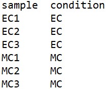Fig14 Fig 13

Note: Enter the sample name in the same order that they are appeared in the ‘Kallisto_out’ folder.

d. Save the file with a file name, say ‘SC_ECvsMC.txt’.

Note: R will usually sort variable conditions alphabetically, and it use the first condition in the list as the control condition. But that won’t work all time. For example, with conditions Mutant and WT; that would make Mutant the control condition. So here, type condition is _WT; the ‘_’ ensures that WT condition is sorted first.

4. R scripting for differential gene expression analysis

Clear the work space
```
rm(list=ls())
```
Load all the required packages

library(sleuth)
library(biomaRt)
library(devtools)
library('ggplot2')

Change the working directory. In this example I keep the kallisto output in ‘D’ drive with a folder name ‘Sleuth_analysis’.
```
setwd('D:/Sleuth_analysis')
```
Provide the path of kallisto output. Here I place the kallisto output in the folder Kallisto_out
```
base_dir <- 'D:/Sleuth_analysis/Kallisto_out'
```
Get the sample names from the Kallisto_out folder.
```
sample_id <- dir(file.path(base_dir))
```

Get the path of each sample by using ‘sample_id’

kal_dirs <- sapply(sample_id, function(id) file.path(base_dir, id))

Read the sample-condition table, which is we already made in text file and stored in ‘Sleuth_analysis’ folder
```
s2c <- read.table("SC_ECvsMC.txt", header = TRUE, stringsAsFactors=FALSE)
```
Add a column to s2c that locate the directories of each sample.

s2c <- dplyr::mutate(s2c, path = kal_dirs)

s2c

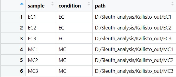Fig15 Fig 14 s2c

Kallisto output has only transcripts, and no information about genes. Gene information can be added which allowing for searching and analysis by gene name instead of transcript.We can collect gene names from Ensembl

mart <- useMart(biomart = "ENSEMBL_MART_ENSEMBL", dataset = "dmelanogaster_gene_ensembl", host="uswest.ensembl.org",ensemblRedirect = FALSE)

Note: We need internet connection to run this code. Sometime host may be unresponsive. If the above code is not working, then use the alternate code;

mart <- useEnsembl(biomart = "ensembl", dataset = "dmelanogaster_gene_ensembl"))

Convert transcript to gene

t2g <-biomaRt::getBM(attributes = c("ensembl_transcript_id", "ensembl_gene_id","external_gene_name"), mart = mart)

t2g <- dplyr::rename(t2g, target_id = ensembl_transcript_id,ens_gene = ensembl_gene_id, ext_gene = external_gene_name)

Construct the sleuth object and add gene name into the sleuth table. Sleuth object contains the information about the experiment, details of the model to be used for differential testing, and the results.

so<- sleuth_prep(s2c, ~ condition, target_mapping = t2g,aggregation_column = 'ext_gene', gene_mode = TRUE, extra_bootstrap_summary=T,
                 read_bootstrap_tpm = TRUE)

fitting the full model and estimate parameters for the sleuth response error measurement model.
```
so <- sleuth_fit(so, ~condition, "full")
```

In this example we have only one condition, that is cell type (MC or EC). Hence our full model is with read_count ~ condition. As described earlier if we have an additional condition like temperature, full model could be read_count ~ condition1 + condition2, ie read_count ~cell type + temperature. So, in this situation we can define a reduced model with only one condition as follows;

so <- sleuth_fit(so, ~condition1+condition2, "full")
so <- sleuth_fit(so, ~condition1, "reduced")

Now we can test how good is full model compared to reduced model by using likelihood ratio test.

so <- sleuth_lrt(so, "reduced", "full")

Wald test

In our example, we have only one condition (MC or EC). We can use a Wald test to measure the effect of a MC against the EC. Wald tests calculate p values to estimate the significance of any difference between conditions (MC and EC).

First, we have to know what are the models are available for testing:

models(so)

conditionMC

Run Wald tests on ‘conditionMC’

beta='conditionMC'
so <- sleuth_wt(so, which_beta = beta)

Sleuth results

test_table <- sleuth_results(so, beta)
test_table

Fig16 Fig 15

Second column is the gene name, ‘b’ value is the effect sizes which calculates are on the natural log scale. To get the raw effect sizes, take the exponents of the beta values; you could then calculate log2 effect sizes as follows:

test_table$raw_b <- exp(test_table$b)
test_table$log2_b <- log2(test_table$raw_b)

Calculate negative log10 of q value, which can be used for volcano plot.

test_table$neg_log10_qval<- -log10(test_table$qval)

Now we can integrate gene expression of each samples, p, q values of differentially expressed genes, and log2(FC) and write the results to a csv file.

sleuth_gene_matrix <- sleuth_to_matrix(so, 'obs_norm', 'tpm')
sleuth_gene_matrix

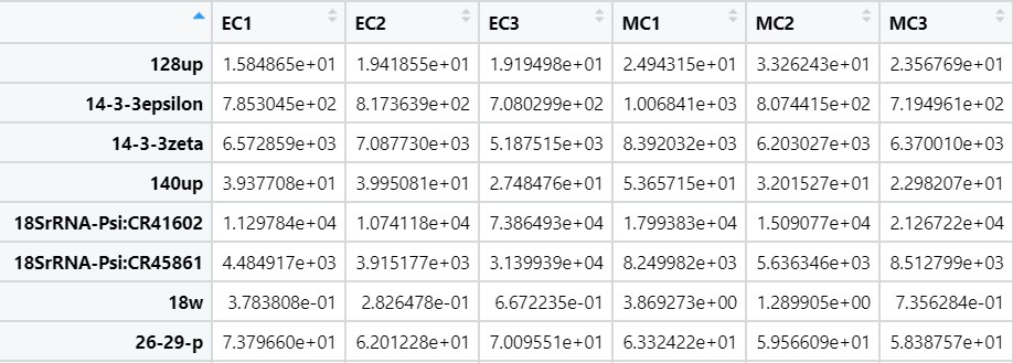Fig 17 Fig 16

Add row names as one colum (gene names)

DGE_table<-cbind(row.names(sleuth_gene_matrix), sleuth_gene_matrix)

Sort test_table according to p value and Extract only genename,p, q and log2(FC)

p_val_sort<-(test_table[order(test_table$target_id),]) 

p_val_reduce<-p_val_sort[c("target_id","pval","qval", "log2_b")]

Megrge with gene expression and p, q and log2(FC)values

DGE_all<-merge(DGE_table, p_val_reduce, by.x=1 , by.y="target_id")

Exclude the NaN value
```
DGE_all<-na.omit(DGE_all)
```

Sort based on FC

DGE_all<-(DGE_all[order(-DGE_all$log2_b),])

Write the results to a csv file

write.csv(DGE_all, 'DGE_table_ECvsMC.csv')

Find the number of differentially expressed genes. Set a q value to find the statistically significant differentially expressed genes. Here we can set q < 0.1 should be significant
```
sig_level=0.1
```
add a column for the significant status

test_table$diffexpressed <- "Not sig"
#if log2Foldchange > 0 and qvalue < 0.1, set as "UP" 
test_table$diffexpressed[test_table$log2_b > 0 & test_table$qval < sig_level] <- "UP"
#if log2Foldchange < 0 qvalue < 0.1, set as "DOWN"
test_table$diffexpressed[test_table$log2_b < 0 & test_table$qval < sig_level] <- "DOWN"

Find the number of differentially expressed, up and down regulated genes

N_significant<-length(test_table$diffexpressed[test_table$diffexpressed !="Not sig"])
N_UP<-length(test_table$diffexpressed[test_table$diffexpressed =="UP"])
N_DOWN<-length(test_table$diffexpressed[test_table$diffexpressed =="DOWN"])

> N_significant
[1] 51
> N_UP
[1] 43
> N_DOWN
[1] 8

Customized volcano plot

ggplot(test_table) + geom_point(aes(x = log2_b, y = neg_log10_qval, col=diffexpressed))+
  geom_vline(xintercept=0, col="black",  linetype="dashed")+
  scale_color_manual(values=c("blue", "black", "red"))+
  labs(x = "log2(FC)", y="-log10(q)", colour="DEG")

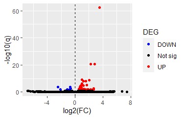Fig18 Fig 17

More analysis and results can be seen on an interactive shiny app by using the following command:

sleuth_live(so)

-Complete R code for RNA seq analysis is below:

rm(list=ls())

library(sleuth)
library(biomaRt)
library(devtools)
library('ggplot2')

setwd('D:/Sleuth_analysis')
base_dir <- 'D:/Sleuth_analysis/Kallisto_out'

sample_id <- dir(file.path(base_dir))
kal_dirs <- sapply(sample_id, function(id) file.path(base_dir, id))
s2c <- read.table("SC_ECvsMC.txt", header = TRUE, stringsAsFactors=FALSE)
s2c <- dplyr::mutate(s2c, path = kal_dirs)

#mart <- useEnsembl(biomart = "ensembl", dataset = "dmelanogaster_gene_ensembl")
mart <- useMart(biomart = "ENSEMBL_MART_ENSEMBL", dataset = "dmelanogaster_gene_ensembl", host="uswest.ensembl.org",ensemblRedirect = FALSE)
t2g <- biomaRt::getBM(attributes = c("ensembl_transcript_id", "ensembl_gene_id","external_gene_name"), mart = mart)
t2g <- dplyr::rename(t2g, target_id = ensembl_transcript_id,ens_gene = ensembl_gene_id, ext_gene = external_gene_name)

so<- sleuth_prep(s2c, ~ condition, target_mapping = t2g,aggregation_column = 'ext_gene', gene_mode = TRUE, extra_bootstrap_summary=T,
                 read_bootstrap_tpm = TRUE)

so <- sleuth_fit(so, ~condition, "full")
models(so)
beta='conditionMC'
so <- sleuth_wt(so, which_beta = beta)

sig_level=0.1
test_table <- sleuth_results(so, beta)
test_table$raw_b <- exp(test_table$b)
test_table$log2_b <- log2(test_table$raw_b)
test_table$neg_log10_qval<- -log10(test_table$qval)
sleuth_gene_matrix <- sleuth_to_matrix(so, 'obs_norm', 'tpm')

DGE_table<-cbind(row.names(sleuth_gene_matrix), sleuth_gene_matrix)# Add row names as one colum (gene names
p_val_sort<-(test_table[order(test_table$target_id),]) # sort according to gene name
p_val_reduce<-p_val_sort[c("target_id","pval","qval", "log2_b")] # extract only genename,p and q and log2()
DGE_all<-merge(DGE_table, p_val_reduce, by.x=1 , by.y="target_id") # megrge with gene expression and p, q values
DGE_all<-na.omit(DGE_all)
DGE_all<-(DGE_all[order(-DGE_all$log2_b),])
write.csv(DGE_all, 'DGE_table_ECvsMC.csv')

test_table$diffexpressed <- "Not sig"
test_table$diffexpressed[test_table$log2_b > 0 & test_table$qval < sig_level] <- "UP"
test_table$diffexpressed[test_table$log2_b < 0 & test_table$qval < sig_level] <- "DOWN"

N_significant<-length(test_table$diffexpressed[test_table$diffexpressed !="Not sig"])
N_UP<-length(test_table$diffexpressed[test_table$diffexpressed =="UP"])
N_DOWN<-length(test_table$diffexpressed[test_table$diffexpressed =="DOWN"])

N_significant
N_UP
N_DOWN

library('ggplot2')
ggplot(test_table) + geom_point(aes(x = log2_b, y = neg_log10_qval, col=diffexpressed))+
  geom_vline(xintercept=0, col="black",  linetype="dashed")+
  scale_color_manual(values=c("blue", "black", "red"))+
  labs(x = "log2(FC)", y="-log10(q)", colour="DEG")
  
  sleuth_live(so)
  